References·AI & automation·eCommerce

Seasonal sales forecasting for purchasing, production and stock transfers

A weekly evaluation compares both forecasting methods with actual sales for 4,629 products. Historical demand, seasonal patterns and known retail events inform the forecast; bills of materials, stock and expected deliveries then turn it into requirements. Purchasing, production and stock transfers can now choose a forecasting method on measured evidence.

Key facts

Requirements for purchasing, production and transfers use a forecast checked weekly against actual demand for every product across five time windows

The new forecast leads by 4.9 points over 180 days and 13.8 points for days 91 to 180, when long-lead-time purchasing decisions are made

Gross-profit-weighted quantity error falls from 86.3 to 71.4 percent

The limits are quantified: 97.5 percent of the remaining deviation is specific to individual products and cannot be explained by the available sales data

Client

McFilter

Industry

eCommerce

Two forecasts, one benchmark: order quantities can now be evaluated

Purchase suggestions, production orders and transfers to Amazon warehouses depend on one figure: expected demand per product per day. Previously, that figure came from a weighted average of the last 42 selling days, split into three fortnightly blocks and adjusted for days without stock. This works for a stable range. For seasonal products, a six-week average cannot capture an annual pattern.

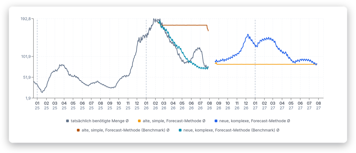
Since May 2026, a second method has run alongside it: TimesFM, a time-series model with 200 million parameters hosted on the company’s own network. A weekend evaluation tests both methods against historical data and shows which was closer for each product. The company’s own sales history determines the result.

Demand forecastingSeasonalityLocally hosted time-series modelForecast benchmarkingPurchase suggestions

Line chart from January 2025 to August 2027: the grey line shows a product’s actual requirements with a recurring annual pattern and a pronounced winter peak. In the historical view, the new forecast follows the decline while the old method stays flat above it. Looking ahead, the new forecast predicts another seasonal peak while the old method remains a flat line.

The starting point: a rolling average without seasonality

A forecast becomes an order, and an order cannot be recalled at short notice. If the estimate is too low, a product may be unavailable for weeks; if it is too high, capital sits in the warehouse. In August 2026, McFilter prioritised cost transparency and seasonality. The reason was clear: the statistical model could not keep up with rapid sales growth, and stock ran short.

The simple method looks back 42 days and projects a constant daily value; its own job description states that seasonal and long-term trends are not considered

Product 420111804 on 3 June 2026: actual requirement 118.9 units, complex forecast 64.3, simple forecast 136.5. One method substantially underestimates demand, the other moderately overestimates it

Promotions, price changes and competitors’ responses affect sales but are not represented in the company’s data

Without a common benchmark, there was no way to decide which method was better for which product

The turning point: from historical sales to operational demand planning

Established reliable historical demand

Days without saleable stock are excluded so that stockouts do not appear as weak demand. Individual marketplace listings often sell too infrequently to support a stable forecast. The model therefore works with sufficiently large product groups and allocates the result back to listings using their share of sales over the last 42 days.

Modelled seasonality and retail events

Annual patterns come from the groups’ sales history. The German retail calendar adds known influences: public holidays, Black Friday, Cyber Week, Advent, Christmas and Easter periods become forecast features.

Forecast and measured future sales

An evaluation moves the forecast start 180 days into the past, reruns the 42-day baseline and time-series model, and compares both with subsequent actual sales. Quantity error and error direction produce an order score for each product and time window. During integration, we found four corrections applied only to the evaluated branch while the branch calculating order quantities remained uncorrected. Sharing one implementation doubled the measured lead from 1.78 to 3.66 points.

Translated sales into requirements

Expected sales feed directly into requirements. Sets and bills of materials break demand down into the necessary components; current stock and expected deliveries complete the requirement signal.

Prepared operational decisions

Purchasing, production and FBA transfers use the same expected demand. Business users can compare methods and inspect results before purchase, production or transfer suggestions are created. We implemented and measured a switch to the simple method for fast-growing products. It helped the example product but worsened the overall forecast, so it was not put into production.

Both methods run side by side in production; orders still use the simple method. McFilter decides when to switch based on the measured results. Technically, the switch is an application setting.

4,629

products with forecasts evaluated every week

Improved ordering accuracy

Traceable down to the formula

The interface explains quantity error, error direction and order score, including the relative weighting of shortages and excess stock. Anyone questioning a result can inspect the calculation.

Identifiable outliers

Every product in the table opens individually, showing sales history, both forecast curves and the groups used to calculate its value.

The original problem case, measured

Product 420111804, whose shortage triggered the investigation, now scores more than 19 points above the old method. Its error direction is plus 4.1 rather than plus 58.2 percent.

Known limits

A perfect group forecast would be worth just 1.37 points. The next improvement therefore depends on promotion and pricing data, rather than a different model.

McFilter

McFilter has sold vacuum cleaner bags and accessories through the major online marketplaces since 2004. Based in Ebersbach-Neugersdorf in Saxony, the company handles product development, purchasing, warehousing and shipping in-house.

Two tenants cover 39 active sales channels across Amazon, eBay, other marketplaces and the company’s own shops, generating around 910,000 orders over twelve months. Unimatrix combines these data with inventory management and logistics to support reporting, profitability analysis and planning, from purchasing through production to transfers into Amazon warehouses.

Visit McFilter’s website

Customer story: McFilter